Transportation Engineering is worth 9 to 14 questions on the 110-question FE Civil exam, so it carries about as much weight as any single knowledge area you will see. The problems are mostly geometric design and traffic operations: lay out a horizontal curve, size a crest vertical curve for stopping sight distance, check a superelevation rate, or convert a counted volume into a rate of flow.
The practice problems below follow that same mix. Each one is solved the way you would solve it at Pearson VUE: find the equation in the Transportation chapter of the handbook, confirm what units it expects, then run the numbers. Work them with a calculator and the on-screen handbook open, not with a formula sheet you wrote out yourself.
Exam weight: NCEES lists Transportation Engineering at 9-14 questions of the 110-question FE Civil exam. Work each problem below on paper first, then reveal the worked solution — reading a solution you have not attempted builds recognition, not recall.
What NCEES Tests in Transportation Engineering
The NCEES specification splits this area into geometric design, traffic operations and capacity, and transportation planning. Geometric design dominates: horizontal curve elements T, L, M, E and the long chord, stationing of the PC and PT, degree of curve, crest and sag vertical curves through the K value, sight distance across a horizontal curve, and the superelevation relationship e plus f equals V squared over 15R.
The traffic side includes stopping and intersection sight distance, the Greenshields linear speed-density model, the flow equals density times speed relationship, peak hour factor, level of service inputs, signal timing components such as the yellow change and all-red intervals, and crash rates per million entering vehicles. Pavement questions stay at the level of layer thickness, structural number, and basic flexible versus rigid behavior.
5 Free Transportation Engineering Practice Problems
Each transportation engineering problem below comes from the FEExamClick FE Civil question bank, with worked solutions, and matches the style, difficulty and format of the real exam. Attempt each one under a three-minute limit — roughly the pace the exam demands.
Problem 1 — A. Geometric design (e.g., streets, highways, intersections)
A car is traveling \( 45\,\mathrm{mph} \). If perception-reaction time is \( 2.0\,\mathrm{s} \), what is the reaction distance (\( \mathrm{ft} \)), using \( d = 1.47 V t \)?
Answer: D) \( 132\,\mathrm{ft} \)
Step 1 – Identify given information: Speed \( V = 45 \;\text{mph} \), perception-reaction time \( t = 2.0 \;\text{s} \).
Step 2 – Reaction distance formula: The distance traveled during perception-reaction time before braking begins:
$$d = 1.47Vt$$
The factor \( 1.47 \) converts mph to ft/s (\( 1 \;\text{mph} = 1.467 \;\text{ft/s} \)).
Step 3 – Substitute and solve:
$$d = 1.47 \times 45 \times 2.0 = 132.3 \;\text{ft} \approx 132 \;\text{ft}$$
Step 4 – Answer: \( d \approx 132 \;\text{ft} \). During the 2-second reaction time, the vehicle travels 132 ft at constant speed before the driver applies brakes. This is independent of grade or friction.
Option (A) is what you get by dividing the speed-time product by 1.47 instead of multiplying - running the mph-to-ft/s conversion backwards.
Correct answer: (D)
Problem 2 — B. Pavement system design (e.g., thickness, subgrade, drainage, rehabilitation)
Use the fourth-power approximation for a single axle: \( LEF = (W/18000)^4 \), where \( W \) is axle load in \( \mathrm{lb} \). What is \( LEF \) for \( W = 16{,}000 \,\mathrm{lb} \) (nearest \( 0.01 \))?
Answer: A) \( 0.62 \)
Step 1 – Identify given information: Axle load \( W = 16{,}000 \;\text{lb} \), standard axle load \( = 18{,}000 \;\text{lb} \).
Step 2 – Fourth-power approximation: The load equivalency factor for a single axle is:
$$LEF = \left(\dfrac{W}{18{,}000}\right)^4$$
This shows that pavement damage increases with the fourth power of the load ratio.
Step 3 – Substitute and solve:
$$LEF = \left(\dfrac{16{,}000}{18{,}000}\right)^4 = (0.8889)^4 = 0.624 \approx 0.62$$
Step 4 – Answer: \( LEF \approx 0.62 \). A 16-kip axle causes only 62% of the damage of the standard 18-kip axle. This illustrates the extreme sensitivity of pavement damage to load: even a small overload causes disproportionate damage.
Option (D) is what you get by flipping the ratio and raising \(18{,}000/16{,}000\) to the fourth power instead of \(16{,}000/18{,}000\).
Correct answer: (A)
Problem 3 — C. Traffic capacity and flow theory
A lane follows the Greenshields model with \( S_f = 55 \,\mathrm{mph} \) and \( D_j = 110 \,\mathrm{veh/mi/ln} \). What is the flow when the density is \( 40 \,\mathrm{veh/mi/ln} \)?
Answer: C) \( 1{,}400\,\mathrm{veh/hr/ln} \)
Step 1 – Identify given information: \( S_f = 55 \,\mathrm{mph} \), \( D_j = 110 \,\mathrm{veh/mi/ln} \), \( D = 40 \,\mathrm{veh/mi/ln} \). Step 2 – Greenshields speed and flow (FE Handbook, p. 312): \( S = S_f - \dfrac{S_f}{D_j}D \) and \( V = S_fD - \dfrac{S_f}{D_j}D^2 \), which is the same thing as \( V = SD \). Step 3 – Solve: \( S = 55 - \dfrac{55}{110}(40) = 55 - 20 = 35 \,\mathrm{mph} \); \( V = SD = 35 \times 40 = 1{,}400 \,\mathrm{veh/hr/ln} \). The direct line gives the same: \( 55(40) - 0.5(40)^2 = 2{,}200 - 800 = 1{,}400 \). Step 4 – Answer: \( V = 1{,}400 \,\mathrm{veh/hr/ln} \), option (C). Option (D) is \( S_fD \), the flow if every vehicle still moved at the free-flow speed; the second term is what the density costs. Option (B) uses the optimum speed \( S_f/2 \) regardless of the density, and option (A) subtracts the density from the speed as if they shared units. Correct answer: (C)
Problem 4 — A. Geometric design (e.g., streets, highways, intersections)
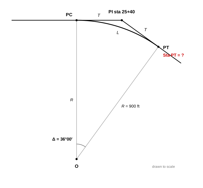
A horizontal curve has \( PI \) at \( \text{sta } 25+40 \), radius \( R = 900 \,\mathrm{ft} \), and intersection angle \( \Delta = 36^{\circ} 00' \). What is the station of \( PT \) (nearest \( 1 \,\mathrm{ft} \))?
Answer: B) \( \text{sta } 28+13 \)
Step 1 – Identify given information:
PI at sta 25+40 (\( 2540.0 \) ft), \( R = 900 \) ft, \( \Delta = 36^{\circ}00' \).
Step 2 – Locate the PC (back along the tangent):
$$T = R\,\tan\!\left(\dfrac{\Delta}{2}\right) = 900\,\tan(18^{\circ}) = 292.4 \;\text{ft}$$
$$\text{sta PC} = 2540.0 - 292.4 = 2247.6 \;\text{ft} = \text{sta } 22+47.6$$
Step 3 – Curve length:
$$L = R\,\Delta_{rad} = 900\,(36^{\circ})\!\left(\dfrac{\pi}{180^{\circ}}\right) = 565.5 \;\text{ft}$$
Step 4 – Station of PT (forward along the curve):
$$\text{sta PT} = \text{sta PC} + L = 2247.6 + 565.5 = 2813.1 \;\text{ft} = \text{sta } 28+13.1 \approx \text{sta } 28+13$$
Option (C) \( 28+32 \) is the classic trap \( PT = PI + T \): stationing runs along the route (the curve), and the PI is not on the route — never station through it.
Correct answer: (B)
Problem 5 — A. Geometric design (e.g., streets, highways, intersections)
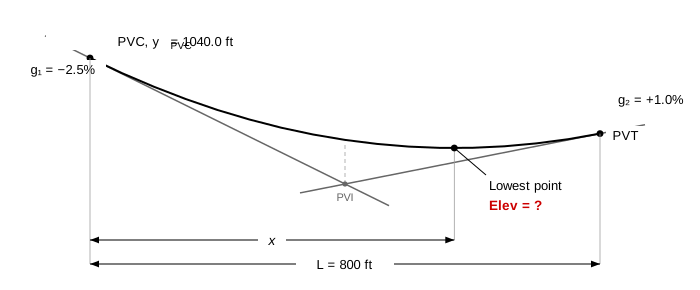
A sag vertical curve has PVC elevation \( y_{PVC} = 1040.0 \,\mathrm{ft} \), length \( L = 800 \,\mathrm{ft} \), \( g_1 = -2.5\% \), and \( g_2 = +1.0\% \). What is the elevation at the lowest point (\( \mathrm{ft} \)), nearest \( 0.1 \,\mathrm{ft} \)?
Answer: B) \( 1032.9\,\mathrm{ft} \)
Step 1 – Identify given information:
\( y_{PVC} = 1040.0 \) ft, \( L = 800 \) ft, \( g_1 = -2.5\% \), \( g_2 = +1.0\% \).
Step 2 – Locate the lowest point:
The grade along the parabola varies linearly and is zero at the low point:
$$x = \dfrac{-g_1 L}{g_2 - g_1} = \dfrac{-(-0.025)(800)}{0.035} = 571.4 \;\text{ft from the PVC}$$
Step 3 – Elevation from the curve equation:
$$y = y_{PVC} + g_1 x + \dfrac{g_2 - g_1}{2L}\,x^2$$
$$y = 1040.0 + (-0.025)(571.4) + \dfrac{0.035}{1600}(571.4)^2 = 1040.0 - 14.29 + 7.14 = 1032.9 \;\text{ft}$$
Step 4 – Answer: \( 1032.9 \) ft. Note the structure: the tangent alone would drop the roadway \( 14.3 \) ft, and the parabolic term recovers exactly half of that (\( +7.1 \) ft) at the point of zero grade.
Correct answer: (B)
Using the FE Reference Handbook for Transportation Engineering
Everything you need sits in the Transportation chapter, but the search box matches words, not symbols. Search sight distance and vertical curve before exam day so you already know the two crest-curve equations appear as a pair, one for S less than L and one for S greater than L. Bookmark the horizontal curve figure; its geometry labels save more time than the formulas do.
Four Mistakes That Cost Points
- Skipping the S versus L check Crest and sag curve length equations come in pairs, one valid when the sight distance is shorter than the curve and one when it is longer. Assume a case, compute L, then verify the assumption actually held. If it did not, redo it with the other equation.
- Losing the 1.47 conversion Speed appears in miles per hour in some handbook equations and feet per second in others. The reaction term of stopping sight distance uses 1.47Vt with V in mph. Write units beside every number before multiplying; unit slips cost more points on this topic than concept errors do.
- Mishandling grade signs in sight distance Grade enters stopping sight distance as a decimal added to or subtracted from the friction term, and a downgrade lengthens the required distance. Entering a 3 percent downgrade as minus 3 instead of minus 0.03 produces an answer that is off by orders of magnitude yet still looks plausible.
- Stationing the curve from the wrong point The PC station is the PI station minus the tangent length T, but the PT is the PC plus the curve length L, not the PI plus T. Adding T twice is the single most common arithmetic error in horizontal curve layout problems, and it matches a distractor.
Frequently Asked Questions
How many transportation questions are on the FE Civil exam?
NCEES lists 9 to 14 questions for Transportation Engineering out of 110. That places it among the larger civil-specific areas. Because the topics repeat in predictable forms, horizontal curves, vertical curves, and sight distance above all, it is one of the better areas to over-prepare relative to the study time it costs.
Do I need the AASHTO Green Book for FE transportation problems?
No. Every design value and equation you are expected to use is reproduced in the NCEES FE Reference Handbook, which is the only reference available on screen at the test center. Studying from the Green Book is not wrong, but practice with the handbook's own notation and table layout so nothing looks unfamiliar while the clock is running.
What is the difference between degree of curve by arc and by chord?
The arc definition is the central angle subtended by a 100-foot arc; the chord definition uses a 100-foot chord. Highway work uses the arc definition, and that is what the handbook provides, with D equal to 5729.58 divided by R. Read the problem statement carefully, since a chord-defined value changes R slightly on large-radius curves.
How much traffic flow theory do I actually need?
Enough to use the fundamental relationship flow equals density times speed, and the Greenshields linear speed-density model, including locating capacity at half the free-flow speed and half the jam density. You should also apply a peak hour factor to convert an hourly volume into a rate of flow. Detailed Highway Capacity Manual procedures are not tested at this level.
Keep Going
Done with transportation engineering? Work through the other FE Civil knowledge areas with more free practice problems, review the full FE Civil exam topic breakdown, or plan your preparation with our FE exam study guide and study timeline. Or test yourself against the clock with the free FE Civil practice exam: 20 timed questions in the CBT format.